Lab 1

Overview

This lab covers three primary topics: (a) working with git and GitHub collaboratively, (b) creating basic visualizations, and (c) working with textual data.You should plan to work together with your group.

The basics of the lab are to:

• Create a shared repo

• Download a whole bunch of data from a github repo (https://github.com/datalorax/edld652)

• Work on different pieces of the lab together

  • File issues for the different pieces of the lab
  • Create branches for those issues
  • Different people work on different branches - merge them in when you’re ready

• Submit a link to the repo through Canvas when you’ve completed the lab

• I check the commit history, and give each person credit

To receive full credit you must create and merge branches. The contributions across team members should also appear roughly equal.

Data

*We will learn to explore some data from the Department of Education for the first part of this lab that we saw in the class slides (https://github.com/datalorax/edld652)

*We’ll then work with Week 1 of the #tidytuesday data for 2019, specifically the #rstats dataset, containing nearly 500,000 tweets over a little more than a decade using that hashtag. The data is in the data folder of the course repo.

Installing edld652 data package

• Install with

remotes::install_github("datalorax/edld652", force = TRUE)

Check to see if all is working

After you’ve done everything on the prior slide, run the following to make sure it’s working

library(edld652)
list_datasets()

Accessing a dataset

• The list_datasets() function shows you a list of all available datasets

• You can import any of these into R with the get_data() function by passing the name of the dataset as a string.

For example: Average cohort graduate rates for local education agency data, 2011 to 2019

acgd <- get_data("EDFacts_acgr_lea_2011_2019")
# acgd

Accessing documentation

• The names of the datasets themselves can sometimes be a bit cryptic

• The variable names are often not interpretable at all (particularly the financial data)

• You can access the documentation for any dataset with the get_documentation() function, again passing the name of the dataset

• This function operates slightly differently on Mac/Windows

• Mac

  • Creates a folder in your current working directory called data-documentation
  • Downloads the documentation and places it in that folder
  • Opens the documentation
  • If the same documentation is requested again, skip the download and just open

• Windows

  • Prints a link to your console where documentation can be downloaded

acgdd <- get_documentation("EDFacts_acgr_lea_2011_2019")
# acgdd

Now let’s move on to the next Data

We’ll now work with Week 1 of the #tidytuesday data for 2019, specifically the #rstats dataset, containing nearly 500,000 tweets over a little more than a decade using that hashtag. The data is in the data folder of the course repo. Start with grabbing that data.

In this part of the lab you will do:

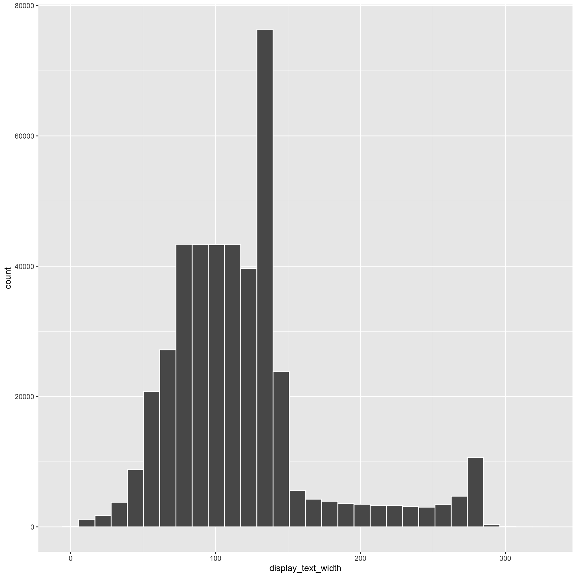
• Initial explorations of the display_text_width variable, including different binning methods.

• Final versions of each of the two plots

1. Initial exploration

Create histograms and density plots of the display_text_width. Try at least four different binning methods and select what you think best represents the data for each. Provide a brief justification for your decision.

2. Look for “plot”

Search the text column for the work “plot”. Report the proportion of posts containing this word.

3. Plot rough draft

Create the following figure of the 15 most common words represented in the posts.

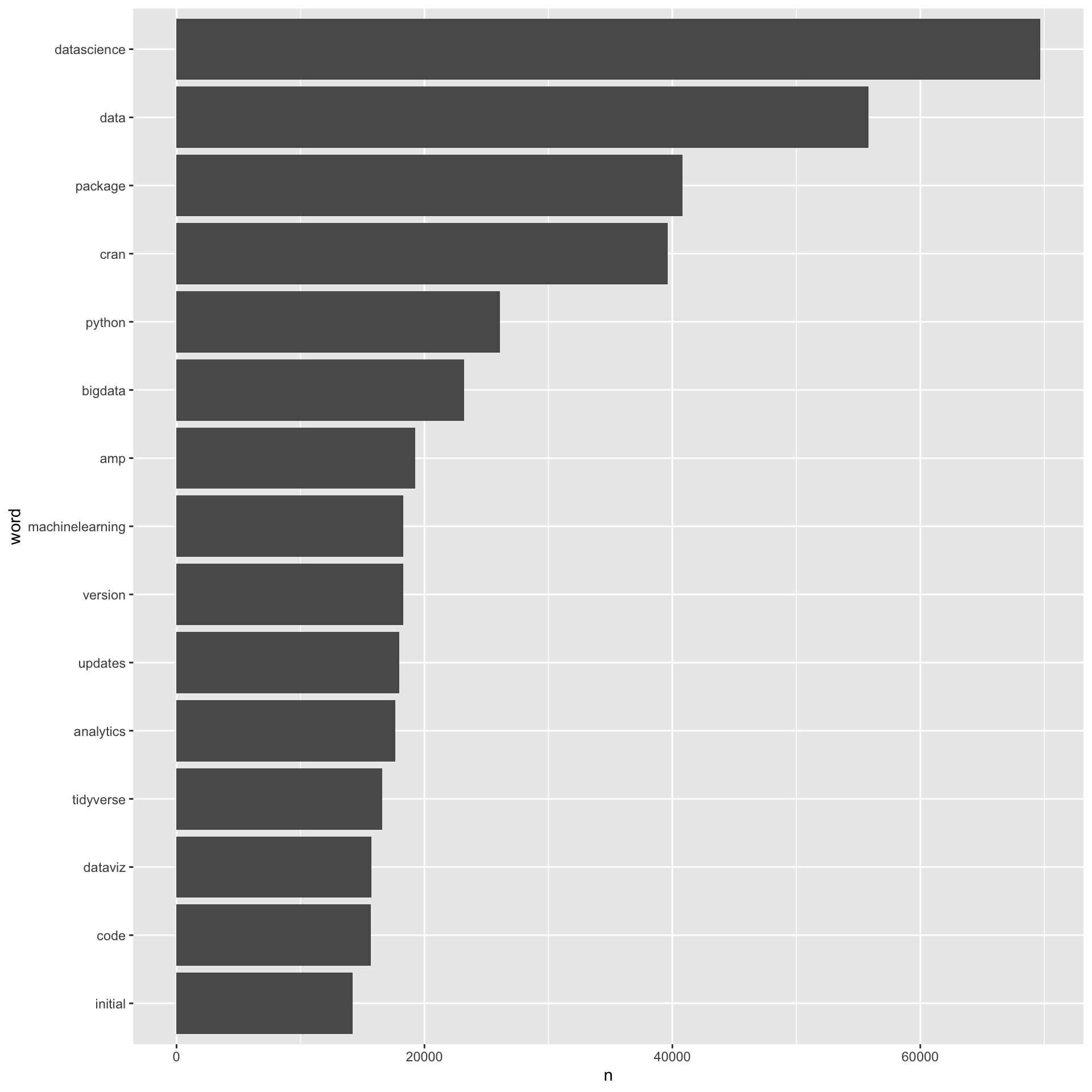
Some guidance

• You’ll need to drop a few additional words beyond stop words to get a clear picture as above. Consider removing rows where the word is not %in% c("t.co", "https", "http", "rt", "rstats"). This can be a bit tricky (see here for additional help)

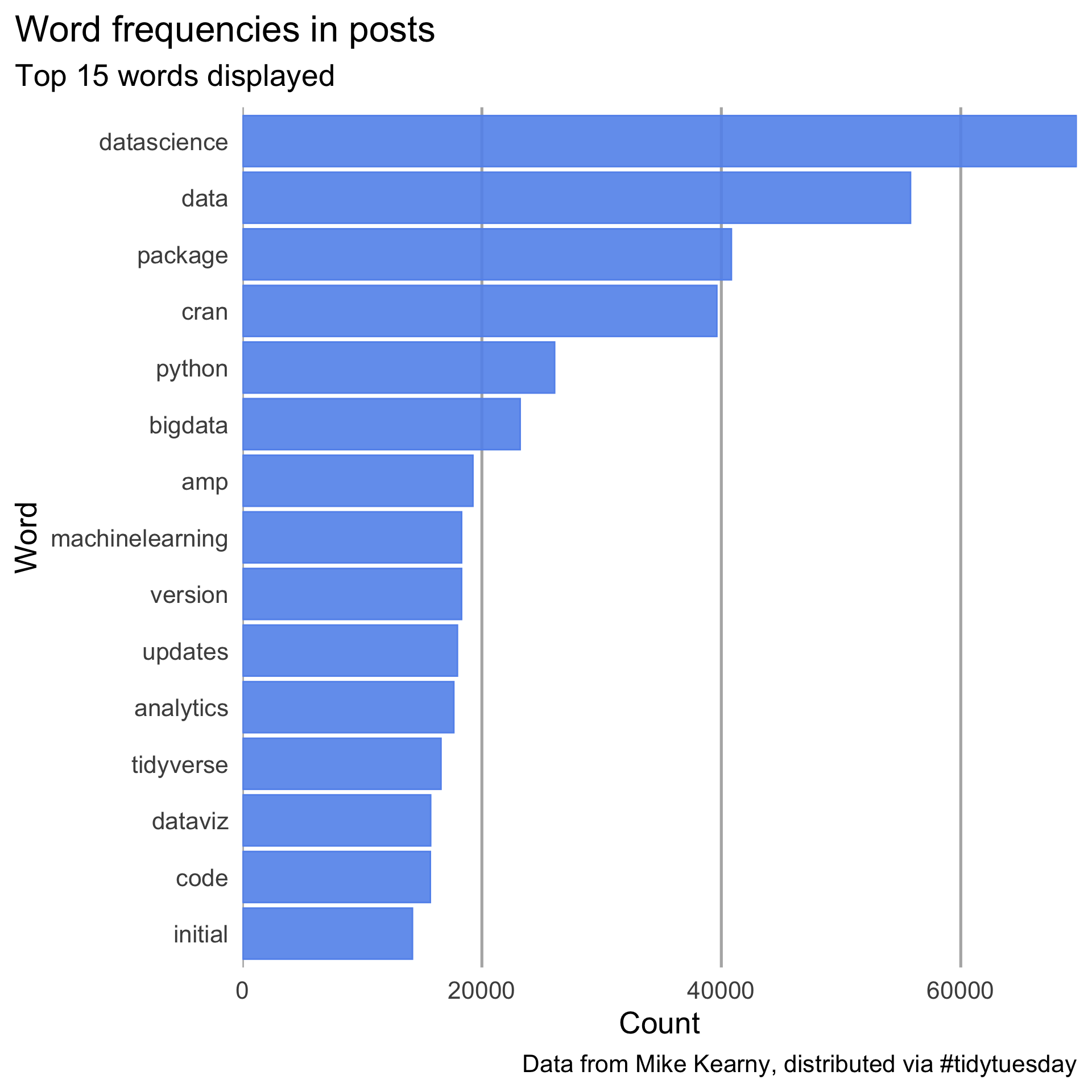
4. Stylized Plot

Style the plot so it (mostly) matches the below. It does not need to be exact, but it should be close.

Finishing up

It is expected that this lab will take you more time than we will devote to it in class. Class time should be used to clarify any points of confusion and if you run into issues after class, please get in touch with me so we can arrange a time to meet and I can help you.

Once you have finished, please go to Canvas and submit a link to your shared repo. Credit will be awarded based on the commit history.